Attēls:VFPt dipoles electric.svg

Kopsavilkums
| Apraksts |
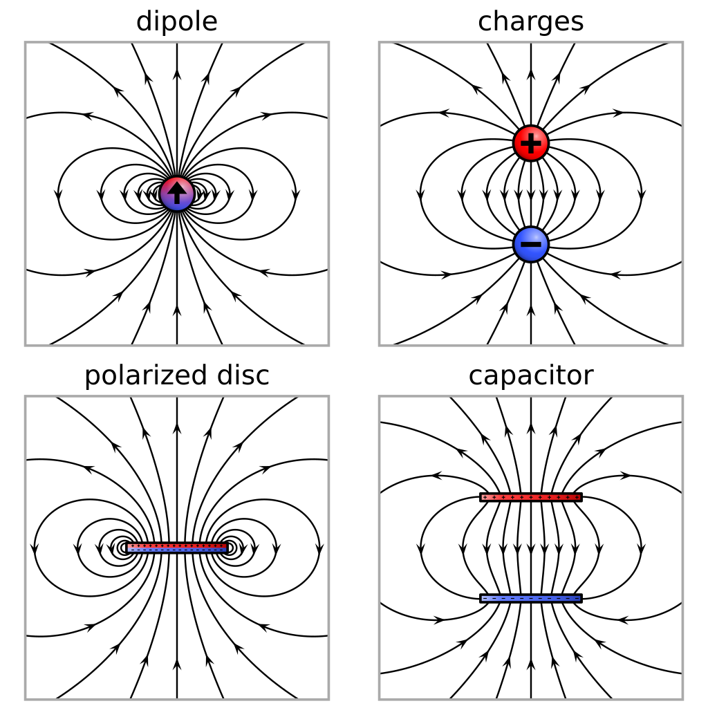
English: Computed drawings of four different types of electric dipoles.
Upper left: An ideal point-like dipole. The field shape is scale invariant and approximates the field of any charge configuration with nonzero dipole moment at large distance. Русский: Рассчитанные электростатические поля четырех различных типов электрических диполей.
Поле идеального точечного диполя. Конфигурация поля в большом масштабе инвариантна и приблизительно соответствует полю любой конфигурации зарядов с ненулевым дипольным моментом на большом расстоянии. Дискретный диполь двух противоположных точечных зарядов разнесенных на конечное расстояние, – физический диполь. Тонкий круглый диск с равномерной электрической поляризацией вдоль оси симметрии. Плоский конденсатор с одинаково заряженными круглыми обкладками. Несмотря на различие этих конфигураций, вблизи которых поля существенно различаются, все эти поля сходятся к одному и тому же дипольному полю на больших расстояниях где они приблизительно одинаковы, при этом любая система зарядов может моделировать идеальный электрический диполь. |
| Datums | |
| Avots | Paša darbs |
| Autors | Geek3 |
| Citas versijas |
|
| SVG veidošana | switch elements: all translations are stored in the same file. |
| Pirmkods | Python code# paste this code at the end of VectorFieldPlot 3.3
R = 0.6
h = 0.6
rsym = 21
doc = FieldplotDocument('VFPt_dipoles_electric1', commons=True,
width=360, height=360)
field = Field([ ['dipole', {'x':0, 'y':0, 'px':0., 'py':1.}] ])
def f_arrows(xy):
return xy[1] * (sc.hypot(xy[0], xy[1]) / 1.4 - 1)
def f_cond(xy):
return hypot(*xy) > 1e-4 and (fabs(xy[1]) < 1e-3 or fabs(xy[1]) > .3)
nlines = 19
startpoints = Startpath(field, lambda t: 0.25*sc.array([sin(t), cos(t)]),
t0=-pi/2, t1=pi/2).npoints(nlines)
for p0 in startpoints:
line = FieldLine(field, p0, directions='both')
doc.draw_line(line, maxdist=1, arrows_style={'at_potentials':[0.],
'potential':f_arrows, 'condition_func':f_cond, 'scale':1.2})
# draw dipole symbol
rb_grad = etree.SubElement(doc._get_defs(), 'linearGradient')
rb_grad.set('id', 'grad_rb')
for attr, val in [['x1', '0'], ['x2', '0'], ['y1', '0'], ['y2', '1']]:
rb_grad.set(attr, val)
for col, of in [['#3355ff', '0'], ['#9944aa', '0.5'], ['#ff0000', '1']]:
stop = etree.SubElement(rb_grad, 'stop')
stop.set('stop-color', col)
stop.set('offset', of)
stop.set('stop-opacity', '1')
symb = doc.draw_object('g', {'id':'dipole_symbol',
'transform':'scale({0},{0})'.format(1./doc.unit)})
doc.draw_object('circle', {'cx':'0', 'cy':'0', 'r':rsym,
'fill':'url(#grad_rb)', 'stroke':'none'}, group=symb)
doc._check_whitespot()
doc.draw_object('circle', {'cx':'0', 'cy':'0', 'r':rsym,
'fill':'url(#white_spot)', 'stroke':'#000000', 'stroke-width':'3'},
group=symb)
doc.draw_object('path', {'fill':'#000000', 'stroke':'none',
'd':'M 3,-12 V 0 H 12 L 0,15 L -12,0 H -3 V -12 H 3 Z'}, group=symb)
doc.write()
doc = FieldplotDocument('VFPt_dipoles_electric2', commons=True,
width=360, height=360)
field = Field([ ['monopole', {'x':0, 'y':h, 'Q':1}],
['monopole', {'x':0, 'y':-h, 'Q':-1}] ])
def f_arrows(xy):
return xy[1] * (sc.hypot(xy[0], xy[1]) / 1.4 - 1)
def f_cond(xy):
return fabs(xy[0]) < 1.4
nlines = 18
stp = Startpath(field, lambda t: R*sc.array([.2*sin(t), 1+.2*cos(t)]),
t0=-pi, t1=pi)
startpoints = [stp.startpos(s) for s in sc.arange(nlines)/float(nlines)]
startpoints.append(startpoints[nlines//2].dot([[1,0],[0,-1]]))
for p0 in startpoints:
line = FieldLine(field, p0, directions='both', maxr=100)
doc.draw_line(line, maxdist=1, arrows_style={'at_potentials':[0.],
'potential':f_arrows, 'condition_func':f_cond, 'scale':1.2})
# draw charge symbols
symb_plus = doc.draw_object('g', {
'transform':'translate(0,{0}) scale({1},{1})'.format(h, 1./doc.unit)})
symb_minus = doc.draw_object('g', {
'transform':'translate(0,{0}) scale({1},{1})'.format(-h, 1./doc.unit)})
for i, g in enumerate([symb_plus, symb_minus]):
doc.draw_object('circle', {'cx':'0', 'cy':'0', 'r':rsym, 'stroke':'none',
'fill':['#ff0000', '#3355ff'][i]}, group=g)
doc._check_whitespot()
doc.draw_object('circle', {'cx':'0', 'cy':'0', 'r':rsym,
'fill':'url(#white_spot)', 'stroke':'#000000', 'stroke-width':'3'}, group=g)
c_symb = doc.draw_object('path', {'fill':'#000000', 'stroke':'none'}, group=g)
if i == 0: # plus sign
c_symb.set('d', 'M 3,3 V 12 H -3 V 3 H -12 V -3'
+ ' H -3 V -12 H 3 V -3 H 12 V 3 H 3 Z')
else: # minus sign
c_symb.set('d', 'M 12,3 H -12 V -3 H 12 V 3 Z')
doc.write()
doc = FieldplotDocument('VFPt_dipoles_electric3', commons=True,
width=360, height=360)
field = Field([ ['ringcurrent', {'x':0, 'y':0, 'R':R, 'phi':pi/2, 'I':1.}] ])
def f_arrows(xy):
return xy[1] * (sc.hypot(xy[0], xy[1]) / 1.4 - 1)
def f_cond(xy):
return hypot(*xy) > 1.2*R and fabs(fabs(xy[0]) - 1.4) > 0.2
nlines = 19
startpoints = Startpath(field, lambda t: sc.array([R*t, 0.]),
t0=-0.9375, t1=0.9375).npoints(nlines)
for p0 in startpoints:
line = FieldLine(field, p0, directions='both')
doc.draw_line(line, maxdist=1, arrows_style={'at_potentials':[0.],
'potential':f_arrows, 'condition_func':f_cond, 'scale':1.2})
# draw polarized sheet
sheet = doc.draw_object('g', {'id':'polarized_sheet'})
s = 0.06
doc.draw_object('rect', {'x':-R, 'y':-s, 'width':2*R, 'height':2*s,
'stroke':'none', 'fill':'#3355ff'}, group=sheet)
doc.draw_object('rect', {'x':-R, 'y':0, 'width':2*R, 'height':s,
'stroke':'none', 'fill':'#ff0000'}, group=sheet)
grad = doc.draw_object('linearGradient', {'id':'grad-round',
'x1':str(R), 'x2':str(-R), 'y1':'0', 'y2':'0',
'gradientUnits':'userSpaceOnUse'}, group=doc.defs)
for o, c, a in ((0, '#000', 0.3), (0.3, '#999', 0.2),
(0.8, '#fff', 0.25), (1, '#fff', 0.65)):
doc.draw_object('stop', {'id':'grad',
'offset':str(o), 'stop-color':c, 'stop-opacity':str(a)}, grad)
doc.draw_object('rect', {'x':-R, 'y':-s, 'width':2*R, 'height':2*s,
'stroke':'#000000', 'stroke-width':0.03, 'fill':'url(#grad-round)',
'stroke-linejoin':'round'}, group=sheet)
symbols_plus = []
symbols_minus = []
for x in sc.linspace(-R*0.875, R*0.875, 16):
symbols_minus.append('M {:.3f},0 h 0.03'.format(x-0.015))
symbols_plus.append('M {:.3f},0 h 0.03 M {:.3f},-0.015 v 0.03'.format(
x-0.015, x))
doc.draw_object('path', {'d':' '.join(symbols_plus), 'stroke':'#000000',
'fill':'none', 'stroke-width':0.01, 'stroke-linecap':'butt',
'transform':'translate(0,0.025)'}, group=sheet)
doc.draw_object('path', {'d':' '.join(symbols_minus), 'stroke':'#000000',
'fill':'none', 'stroke-width':0.01, 'stroke-linecap':'butt',
'transform':'translate(0,-0.025)'}, group=sheet)
doc.write()
doc = FieldplotDocument('VFPt_dipoles_electric4', commons=True,
width=360, height=360)
field_D = Field([ ['coil', {'x':0, 'y':0, 'phi':pi/2, 'R':R, 'Lhalf':h,
'I':1./(R**2*pi)}] ])
field_E = Field([ ['charged_disc', {'x0':-R, 'x1':R, 'y0':h, 'y1':h, 'Q':.5/h}],
['charged_disc', {'x0':-R, 'x1':R, 'y0':-h, 'y1':-h, 'Q':-.5/h}] ])
field_E_inside = Field([ ['homogeneous', {'Fx':0., 'Fy':-.5/(h*R**2*pi)}],
['coil', {'x':0, 'y':0, 'phi':pi/2, 'R':R, 'Lhalf':h, 'I':1./(R**2*pi)}] ])
def f_arrows(xy):
return xy[1] * (sc.hypot(xy[0], xy[1]) / 1.4 - 1)
def f_cond(xy):
return True
# Use fieldlines in D-field to find good starting points
nlines = 13
startpoints = []
startpoints2 = []
for iline in range(nlines):
p0 = sc.array([R * (-1. + 2. * (iline + 0.5) / nlines), 0.])
print('p0', p0)
line_D = FieldLine(field_D, p0, directions='forward',
maxr=100, stop_funcs=2*[lambda xy: -xy[1] - max(0, 1-hypot(*xy)/R)])
p1 = line_D.nodes[-1]['p']
startpoints.append(p1)
if iline >= 3 and iline < nlines - 3:
line_D = FieldLine(field_D, p0, directions='forward',
maxr=2, stop_funcs=2*[lambda xy: xy[1] - h])
p2 = line_D.nodes[-1]['p']
startpoints2.append(p2)
startpoints.append([0, -3])
for p0 in startpoints:
line = FieldLine(field_E, p0, directions='both', maxr=100)
doc.draw_line(line, maxdist=1, arrows_style={'at_potentials':[0.],
'potential':f_arrows, 'condition_func':f_cond, 'scale':1.2})
for p0 in startpoints2:
line = FieldLine(field_E_inside, p0, directions='forward',
stop_funcs=2*[lambda xy: -xy[1] - h])
doc.draw_line(line, maxdist=1, arrows_style={'at_potentials':[0.],
'potential':f_arrows, 'condition_func':f_cond, 'scale':1.2})
# draw charged discs
disc_plus = doc.draw_object('g', {'id':'disc_plus',
'transform':'translate(0,{0})'.format(h)})
disc_minus = doc.draw_object('g', {'id':'disc_minus',
'transform':'translate(0,{0})'.format(-h)})
s = 0.045
grad = doc.draw_object('linearGradient', {'id':'grad-round',
'x1':str(R), 'x2':str(-R), 'y1':'0', 'y2':'0',
'gradientUnits':'userSpaceOnUse'}, group=doc.defs)
for o, c, a in ((0, '#000', 0.3), (0.3, '#999', 0.2),
(0.8, '#fff', 0.25), (1, '#fff', 0.65)):
doc.draw_object('stop', {
'offset':str(o), 'stop-color':c, 'stop-opacity':str(a)}, grad)
for i, g in enumerate([disc_plus, disc_minus]):
doc.draw_object('rect', {'x':-R, 'y':-s, 'width':2*R, 'height':2*s,
'stroke':'none', 'fill':['#ff0000', '#3355ff'][i]}, group=g)
doc.draw_object('rect', {'x':-R, 'y':-s, 'width':2*R, 'height':2*s,
'stroke':'#000000', 'stroke-width':0.03, 'fill':'url(#grad-round)',
'stroke-linejoin':'round'}, group=g)
symbols = []
for x in [R * (2 * (0.5 + isy) / 11 - 1) for isy in range(11)]:
if i == 0:
d = 'M {:.3f},0 h 0.04 M {:.3f},-0.02 v 0.04'.format(x-0.02, x)
else:
d = 'M {:.3f},0 h 0.04'.format(x-0.02)
symbols.append(d)
doc.draw_object('path', {'d':' '.join(symbols), 'stroke':'#000000',
'fill':'none', 'stroke-width':0.01, 'stroke-linecap':'butt'}, group=g)
doc.write()
|


Licence
- Jūs varat brīvi:
- koplietot – kopēt, izplatīt un pārraidīt darbu
- remiksēt – pielāgot darbu
- Saskaņā ar šādiem nosacījumiem:
- atsaucoties – Tev ir jānorāda autors, saite uz licenci un to, vai veiktas kādas izmaiņas. To var darīt jebkādā saprātīgā veidā, bet ne tādā, kas norādītu, ka licencētājs atbalsta tevi vai veidu, kā tu izmanto šo darbu.
- nemainot licenci – Ja tu miksē, pārveido vai izmanto materiālu, tev savs devums jāpublicē ar to pašu vai saderīgu licenci kā oriģināls.
Faila hronoloģija
Uzklikšķini uz datums/laiks kolonnā esošās saites, lai apskatītos, kā šis fails izskatījās tad.
| Datums/Laiks | Attēls | Izmēri | Dalībnieks | Komentārs | |
|---|---|---|---|---|---|
| tagadējais | 2021. gada 22. maijs, plkst. 22.37 | | 840 × 840 (108 KB) | wikimediacommons>Geek3 | added russion captions from VFPt_dipoles_electric-ru.svg |
Faila lietojums
Šo failu izmanto šajā 1 lapā: